

Volume 11, Issue 3 (Summer 2023)
Iran J Health Sci 2023, 11(3): 217-228 |
Back to browse issues page


Download citation:
BibTeX | RIS | EndNote | Medlars | ProCite | Reference Manager | RefWorks
Send citation to:


BibTeX | RIS | EndNote | Medlars | ProCite | Reference Manager | RefWorks
Send citation to:
AL-Husseini Z, Naghizadeh Qomi M, Taghi MirMostafaee S M. Single Acceptance Sampling Plan Based on Truncated-life Tests for the Exponentiated Moment Exponential Distribution With Application in Bladder Cancer Data. Iran J Health Sci 2023; 11 (3) :217-228
URL: http://jhs.mazums.ac.ir/article-1-891-en.html
URL: http://jhs.mazums.ac.ir/article-1-891-en.html


Department of Statistics, Faculty of Mathematical Sciences, University of Mazandaran, Babolsar, Iran. , m.naghizadeh@umz.ac.ir
Full-Text [PDF 1194 kb]
(742 Downloads)
| Abstract (HTML) (1641 Views)
Full-Text: (481 Views)
1. Introduction
Quality control is one of the important applications of the statistical inference method. In this regard, the two important methods are acceptance sampling and control charts. Acceptance sampling is one of the applications of statistical testing in quality control. There are two types of acceptance sampling plans: attributes acceptance sampling plan and variable acceptance sampling plan. In attributes acceptance sampling plans, the decision is based on the number of failures of defectives. In contrast, a variable acceptance sampling plan is used for deciding based on measurements.
A time-truncated sampling plan checks whether a product can be accepted. Due to several constraints like time and cost, checking all products is hardly possible or impossible. Thus, a random sample is drawn from the lot. The test is finished, and the decision is made by a pre-specified time t. Let p* be the consumer’s confidence level, and then the goal is to find a confidence limit on the mean life of products, μ , and to set a specified mean life, μ0 with a probability of at least p*.
The single acceptance sampling plan is the most used attribute acceptance sampling plan, which is simple to use. In this paper, we focus on this type of plan. In a single sampling plan, a lot is accepted if and only if the observed number of failures does not become bigger than c. One can end the test whenever the number of failures gets more than c before the time t and decide to reject the lot. A single sampling plan includes the following parameters:
(i) the number of items on test n,
(ii) the acceptance number c,
(iii) the ratio t/μ0
Figure 1 shows the operation of a single acceptance sampling plan.
.jpg)
This plan has been proposed for many lifetime distributions, for example, the Marshall-Olkin extended Lomax model [1], the generalized exponential model [2], the half-normal model [3], and the exponentiated Frećhet model [4]. Recently, some studies discussed the single sampling plan for the weighted exponential, extended exponential, and power Lomax models [5, 6, 7].
This paper provides a single acceptance sampling plan when the lifetime distribution follows an exponentiated moment exponential (EME) distribution. The EME model was introduced by [8] with the following probability density function (pdf) (Equation 1):
.jpg)
And the corresponding cumulative density function is given by (Equation 2):
.jpg)
Where α>0 and β>0 are the shape and scale parameters, respectively. The EME distribution with parameters α and β is denoted as EMED (α, β). The rth moment of the EME distribution is given by (Equation 3):
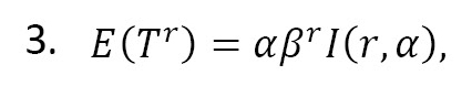
where (Equation 4):

Thus, the mean of the EME distribution is given by (Equation 5):

2. Materials and Methods
Materials
Real data
A real data set regarding the remission times of a random sample of 30 bladder cancer patients (in months) was considered and analyzed. This data set was previously examined in a study [9].
The model used
We assume a parametric model for the lifetime distribution to design a sampling plan. An EME distribution with pdf (1) is used for modeling the bladder cancer data.
Method
Suppose the lifetime follows an EMED (α, β), where α is known. Let μ denote the true average lifetime of a product, and then a lot is considered good if μ ≥ μ0, otherwise, it is considered a bad lot. Thus, the consumer's risk is the probability of accepting a bad lot, whereas the producer’s risk is the probability of rejecting a good one. In this study, we fixed the consumer’s risk to become not greater than P*, where 0 ≤ P*≤ 1. We suppose that the size of the lot is so large that we can use the binomial distribution in our work. The acceptance or rejection of the lot corresponds to the acceptance or rejection of the hypothesis μ ≥ μ0. From (3), we can say that the hypothesis μ ≥ μ0 corresponds to β ≥ β0 where β0=μ0⁄m and m=αI(1,α). The plan is to set a specified time, t and is characterized by the triplet (n, c, t∕μ0), including the number of items n to be drawn from the lot, the acceptance number c and the ratio t∕μ0.
3. Results
Minimum sample size
We estimate the minimum sample size n satisfying the consumer’s risk, the probability of accepting a bad lot, is not to exceed 1-P*, when μ=μ0. The probability of accepting a lot is given by (Equation 6):
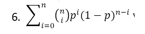
Where p = F(t,α,β) = probability of a failure before time t that is given by p=[1-(1+md)e-md], where d=t⁄μ. For μ=μ0, we have p0=[1-(1+md0) e-md0]α, where d0=t⁄μ0. Therefore, the required n is the smallest positive integer that satisfies the following inequality (Equation 7).
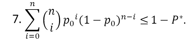
The minimum values of n satisfying (4) are computed and summarized in Tables 1 and 2 for α=0.5,2, P*=0.90, 0.95, 0.99, and d0=0.4, 0.6, 0.8, 1.0, 1.5, 2.0, 2.5, 3.0. Suppose that the remission times (in months) of bladder cancer patients follow the EME distribution with shape parameter α=0.5, and we wish to establish that the mean lifetime is at least 1.39 months with a probability P*=0.95. The life test is terminated at t=2.08 months. Therefore, from Table 1, for d0=1.5 and c=3, the minimum sample size is 8, namely 8 patients should be put on test. If no more than 3 patients fail during 2.08 hours, then the experimenter can assert that the truemean of remission times μ is at least 1.38 months with a confidence level of 0.95.
.jpg)
.jpg)
The shape of the required minimum sample size versus t⁄μ0 for α=2, c=3 , and selected values of the confidence level P* is plotted in Figure 2.
.jpg)
Operating characteristic function
The operating characteristic (OC) function is the probability of accepting a lot. A sampling plan is preferable if its OCs approach more rapidly to one. For the proposed sampling plan (n, c, t∕μ0), the OC is defined as (Equation 8):

Note that increasing the ratio μ⁄μ0 will increase the acceptance probability. Tables 3 and 4 provide the OC function values for the EME distribution adopted from Tables 1 and 2 for c=3, various values of P*, μ⁄μ0 and
α=0.5, 2, respectively. Besides, the values of OC versus μ⁄μ0 are plotted in Figure 3 for α=0.5, t⁄μ0 =0.4 and c=3. From Tables 3 and 4, we observe that the OC function values μ⁄μ0 increase as the ratio increases. If we consider P*=0.95, d0=0.6, c=3 and μ⁄μ0=8, then the sample size is 15 (Table 3), and the OC value is 0.9834.
.jpg)
.jpg)
This outcome reveals that the lot is accepted if less than or equal to 3 patients out of 15 patients fail before time point t=0.83 months and μ ≥ 8μ0=8t∕0.6 =11.07 months, then the lot will be accepted with a probability of at least 0.9834.
.jpg)
Minimum ratio of μ⁄μ0 for the acceptability of a lot
For a specified producer’s risk and a sampling plan (n, c, t∕μ0), one may seek the value of quality level μ⁄μ0 that will ensure the producer’s risk does not become greater than γ. Recall that the producer’s risk is the probability of rejection of a lot when it is good, i.e. μ ≥ μ0 or equivalently β ≥ β0. Then, we seek the minimum values of μ⁄μ0 that satisfy (Equation 9).
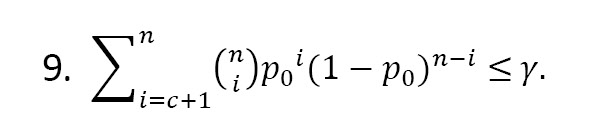
The minimum values of μ⁄μ0 satisfying (6) are presented in Tables 5 and 6 with the producer’s risk of γ=0.05 and α=0.5, 2. Consider a situation where one intends to establish the mean life μ0 is at least 1.39 months with a probability P*=0.95 and desires to end the life test at t=0.83 months. If the actual mean life is μ about 8.33 hours (namely, the value of μ⁄μ0 is around 6), then from Table 5 with the producer’s risk 0.05, we find c=3. We also perceive that the required n in Table 1 corresponds to the values of P*=0.95, c=3, and d0 =0.6 is 15. Hence, a sampling plan (n, c, t∕μ0) =(15, 3, 0.6) may be taken.
.jpg)
.jpg)
Bladder cancer data
In this section, we analyze a real data set from a study [9] regarding the remission times of a random sample of 30 bladder cancer patients (in months):
0.08,0.20,0.40,0.50,0.51,0.81,0.90,1.05,1.19,1.26,1.35,1.40,1.46,1.76,2.02,2.02,2.07,2.09,2.23,2.26,2.46,2.54,2.62,2.64,2.69,2.69,2.75,2.83,2.87,3.02.
We perform a formal Kolmogorov-Smirnov (K-S) test to check if the EME distribution fits the above data well. The K-S statistic is computed as D=0.20217 with the corresponding P that equals 0.1496. The maximum likelihood estimates of the scale and shape parameters are calculated as β ̂=0.8480144 and α ̂=1.0739784, respectively. Thus, we conclude that the two-parameter EME distribution can perfectly model the above data. Figure 4 gives the P-P plot of data.
.jpg)
4. Discussion
The mean lifetime can be estimated as μ ̂=mβ ̂=1.76. If we assume that t=1.06 months, then we get:
Consider P*=0.9, with α=1.07 From Table 7, we obtain n=30 and c=6. Therefore, if the number of patients with remission time before t=1.06 months is less than or equal to 6, we can accept the lot with the assured mean remission of 1.76 and a probability of 0.9. Since the number of patients with remission time before t=1.06 is 8, we can reject the lot.
.jpg)
5. Conclusion
Reliability sampling plans are used to determine the acceptability of a product with respect to its lifetime. Due to various restrictions like time and cost, a complete inspection is impossible. Then, the consumer draws a random sample from the lot, and a decision (acceptance or rejection) is made at a pre-specified time.
In this paper, we developed a single acceptance sampling plan based on the truncated life test for the EME distribution. The minimum sample size required to guarantee a certain mean lifetime of the test items is provided. Two tables and Figure 1 are presented to report the results. A sampling plan is preferable if its OCs approach rapidly to 1. The OC function values are obtained and analyzed in some tables and Figure 1. The results show that the OC function values increase as the ratio μ⁄μ0 increases. Besides, some tables are provided for the minimum ratio of the true mean life to a specified life for the acceptability of a lot with a certain producer’s risk. Moreover, a real data set regarding the remission times of a random sample of 30 bladder cancer patients is provided for illustrative purposes. The K-S test is used for the goodness test of fit for the EME distribution, which shows that EMED (1.0739784,0.8480144) has a good fit to the data. It is noticed here that all computations of this paper were done using statistical software R version 4.2.3 [10]. There were no limitations in this study.
Ethical Considerations
Compliance with ethical guidelines
There were no ethical considerations to be considered in this research.
Funding
The paper was extracted from the PhD. Thesis of Zainalabideen AL-Husseini, Department of Statistics, Faculty of Mathematical Sciences, University of Mazandaran, Babolsar, Iran.
Authors contributions
Investigation and analyses: Zainalabideen, AL-Husseini; Initial idea, writing original draft, methodology, and investigation: Mehran Naghizadeh Qomi; Investigation and editing; Seyed Mohammad Taghi MirMostafaee.
Conflict of interest
The authors declared no conflict of interest.
Acknowledgements
We thank the Editor and the referees for their comments and suggestions on the manuscript.
References
Quality control is one of the important applications of the statistical inference method. In this regard, the two important methods are acceptance sampling and control charts. Acceptance sampling is one of the applications of statistical testing in quality control. There are two types of acceptance sampling plans: attributes acceptance sampling plan and variable acceptance sampling plan. In attributes acceptance sampling plans, the decision is based on the number of failures of defectives. In contrast, a variable acceptance sampling plan is used for deciding based on measurements.
A time-truncated sampling plan checks whether a product can be accepted. Due to several constraints like time and cost, checking all products is hardly possible or impossible. Thus, a random sample is drawn from the lot. The test is finished, and the decision is made by a pre-specified time t. Let p* be the consumer’s confidence level, and then the goal is to find a confidence limit on the mean life of products, μ , and to set a specified mean life, μ0 with a probability of at least p*.
The single acceptance sampling plan is the most used attribute acceptance sampling plan, which is simple to use. In this paper, we focus on this type of plan. In a single sampling plan, a lot is accepted if and only if the observed number of failures does not become bigger than c. One can end the test whenever the number of failures gets more than c before the time t and decide to reject the lot. A single sampling plan includes the following parameters:
(i) the number of items on test n,
(ii) the acceptance number c,
(iii) the ratio t/μ0
Figure 1 shows the operation of a single acceptance sampling plan.
This plan has been proposed for many lifetime distributions, for example, the Marshall-Olkin extended Lomax model [1], the generalized exponential model [2], the half-normal model [3], and the exponentiated Frećhet model [4]. Recently, some studies discussed the single sampling plan for the weighted exponential, extended exponential, and power Lomax models [5, 6, 7].
This paper provides a single acceptance sampling plan when the lifetime distribution follows an exponentiated moment exponential (EME) distribution. The EME model was introduced by [8] with the following probability density function (pdf) (Equation 1):
And the corresponding cumulative density function is given by (Equation 2):
Where α>0 and β>0 are the shape and scale parameters, respectively. The EME distribution with parameters α and β is denoted as EMED (α, β). The rth moment of the EME distribution is given by (Equation 3):
where (Equation 4):
Thus, the mean of the EME distribution is given by (Equation 5):
2. Materials and Methods
Materials
Real data
A real data set regarding the remission times of a random sample of 30 bladder cancer patients (in months) was considered and analyzed. This data set was previously examined in a study [9].
The model used
We assume a parametric model for the lifetime distribution to design a sampling plan. An EME distribution with pdf (1) is used for modeling the bladder cancer data.
Method
Suppose the lifetime follows an EMED (α, β), where α is known. Let μ denote the true average lifetime of a product, and then a lot is considered good if μ ≥ μ0, otherwise, it is considered a bad lot. Thus, the consumer's risk is the probability of accepting a bad lot, whereas the producer’s risk is the probability of rejecting a good one. In this study, we fixed the consumer’s risk to become not greater than P*, where 0 ≤ P*≤ 1. We suppose that the size of the lot is so large that we can use the binomial distribution in our work. The acceptance or rejection of the lot corresponds to the acceptance or rejection of the hypothesis μ ≥ μ0. From (3), we can say that the hypothesis μ ≥ μ0 corresponds to β ≥ β0 where β0=μ0⁄m and m=αI(1,α). The plan is to set a specified time, t and is characterized by the triplet (n, c, t∕μ0), including the number of items n to be drawn from the lot, the acceptance number c and the ratio t∕μ0.
3. Results
Minimum sample size
We estimate the minimum sample size n satisfying the consumer’s risk, the probability of accepting a bad lot, is not to exceed 1-P*, when μ=μ0. The probability of accepting a lot is given by (Equation 6):
Where p = F(t,α,β) = probability of a failure before time t that is given by p=[1-(1+md)e-md], where d=t⁄μ. For μ=μ0, we have p0=[1-(1+md0) e-md0]α, where d0=t⁄μ0. Therefore, the required n is the smallest positive integer that satisfies the following inequality (Equation 7).
The minimum values of n satisfying (4) are computed and summarized in Tables 1 and 2 for α=0.5,2, P*=0.90, 0.95, 0.99, and d0=0.4, 0.6, 0.8, 1.0, 1.5, 2.0, 2.5, 3.0. Suppose that the remission times (in months) of bladder cancer patients follow the EME distribution with shape parameter α=0.5, and we wish to establish that the mean lifetime is at least 1.39 months with a probability P*=0.95. The life test is terminated at t=2.08 months. Therefore, from Table 1, for d0=1.5 and c=3, the minimum sample size is 8, namely 8 patients should be put on test. If no more than 3 patients fail during 2.08 hours, then the experimenter can assert that the truemean of remission times μ is at least 1.38 months with a confidence level of 0.95.
The shape of the required minimum sample size versus t⁄μ0 for α=2, c=3 , and selected values of the confidence level P* is plotted in Figure 2.
Operating characteristic function
The operating characteristic (OC) function is the probability of accepting a lot. A sampling plan is preferable if its OCs approach more rapidly to one. For the proposed sampling plan (n, c, t∕μ0), the OC is defined as (Equation 8):
Note that increasing the ratio μ⁄μ0 will increase the acceptance probability. Tables 3 and 4 provide the OC function values for the EME distribution adopted from Tables 1 and 2 for c=3, various values of P*, μ⁄μ0 and
α=0.5, 2, respectively. Besides, the values of OC versus μ⁄μ0 are plotted in Figure 3 for α=0.5, t⁄μ0 =0.4 and c=3. From Tables 3 and 4, we observe that the OC function values μ⁄μ0 increase as the ratio increases. If we consider P*=0.95, d0=0.6, c=3 and μ⁄μ0=8, then the sample size is 15 (Table 3), and the OC value is 0.9834.
This outcome reveals that the lot is accepted if less than or equal to 3 patients out of 15 patients fail before time point t=0.83 months and μ ≥ 8μ0=8t∕0.6 =11.07 months, then the lot will be accepted with a probability of at least 0.9834.
Minimum ratio of μ⁄μ0 for the acceptability of a lot
For a specified producer’s risk and a sampling plan (n, c, t∕μ0), one may seek the value of quality level μ⁄μ0 that will ensure the producer’s risk does not become greater than γ. Recall that the producer’s risk is the probability of rejection of a lot when it is good, i.e. μ ≥ μ0 or equivalently β ≥ β0. Then, we seek the minimum values of μ⁄μ0 that satisfy (Equation 9).
The minimum values of μ⁄μ0 satisfying (6) are presented in Tables 5 and 6 with the producer’s risk of γ=0.05 and α=0.5, 2. Consider a situation where one intends to establish the mean life μ0 is at least 1.39 months with a probability P*=0.95 and desires to end the life test at t=0.83 months. If the actual mean life is μ about 8.33 hours (namely, the value of μ⁄μ0 is around 6), then from Table 5 with the producer’s risk 0.05, we find c=3. We also perceive that the required n in Table 1 corresponds to the values of P*=0.95, c=3, and d0 =0.6 is 15. Hence, a sampling plan (n, c, t∕μ0) =(15, 3, 0.6) may be taken.
Bladder cancer data
In this section, we analyze a real data set from a study [9] regarding the remission times of a random sample of 30 bladder cancer patients (in months):
0.08,0.20,0.40,0.50,0.51,0.81,0.90,1.05,1.19,1.26,1.35,1.40,1.46,1.76,2.02,2.02,2.07,2.09,2.23,2.26,2.46,2.54,2.62,2.64,2.69,2.69,2.75,2.83,2.87,3.02.
We perform a formal Kolmogorov-Smirnov (K-S) test to check if the EME distribution fits the above data well. The K-S statistic is computed as D=0.20217 with the corresponding P that equals 0.1496. The maximum likelihood estimates of the scale and shape parameters are calculated as β ̂=0.8480144 and α ̂=1.0739784, respectively. Thus, we conclude that the two-parameter EME distribution can perfectly model the above data. Figure 4 gives the P-P plot of data.
4. Discussion
The mean lifetime can be estimated as μ ̂=mβ ̂=1.76. If we assume that t=1.06 months, then we get:
Consider P*=0.9, with α=1.07 From Table 7, we obtain n=30 and c=6. Therefore, if the number of patients with remission time before t=1.06 months is less than or equal to 6, we can accept the lot with the assured mean remission of 1.76 and a probability of 0.9. Since the number of patients with remission time before t=1.06 is 8, we can reject the lot.
5. Conclusion
Reliability sampling plans are used to determine the acceptability of a product with respect to its lifetime. Due to various restrictions like time and cost, a complete inspection is impossible. Then, the consumer draws a random sample from the lot, and a decision (acceptance or rejection) is made at a pre-specified time.
In this paper, we developed a single acceptance sampling plan based on the truncated life test for the EME distribution. The minimum sample size required to guarantee a certain mean lifetime of the test items is provided. Two tables and Figure 1 are presented to report the results. A sampling plan is preferable if its OCs approach rapidly to 1. The OC function values are obtained and analyzed in some tables and Figure 1. The results show that the OC function values increase as the ratio μ⁄μ0 increases. Besides, some tables are provided for the minimum ratio of the true mean life to a specified life for the acceptability of a lot with a certain producer’s risk. Moreover, a real data set regarding the remission times of a random sample of 30 bladder cancer patients is provided for illustrative purposes. The K-S test is used for the goodness test of fit for the EME distribution, which shows that EMED (1.0739784,0.8480144) has a good fit to the data. It is noticed here that all computations of this paper were done using statistical software R version 4.2.3 [10]. There were no limitations in this study.
Ethical Considerations
Compliance with ethical guidelines
There were no ethical considerations to be considered in this research.
Funding
The paper was extracted from the PhD. Thesis of Zainalabideen AL-Husseini, Department of Statistics, Faculty of Mathematical Sciences, University of Mazandaran, Babolsar, Iran.
Authors contributions
Investigation and analyses: Zainalabideen, AL-Husseini; Initial idea, writing original draft, methodology, and investigation: Mehran Naghizadeh Qomi; Investigation and editing; Seyed Mohammad Taghi MirMostafaee.
Conflict of interest
The authors declared no conflict of interest.
Acknowledgements
We thank the Editor and the referees for their comments and suggestions on the manuscript.
References
- Rao GS, Ghitany ME, Kantam RRL. Acceptance sampling plans for Marshall-Olkin extended Lomax distribution. International Journal of Applied Mathematics. 2008; 21(2): 315-25. [Link]
- Aslam M, Kundu D, Ahmad M. Time truncated acceptance sampling plans for generalized exponential distribution. Journal of Applied Statistics. 2010; 37(4):555-66. [DOI:10.1080/02664760902769787]
- Lu X, Gui W, Yan J. Acceptance sampling plans for half normal distribution under truncated life tests. American Journal of Mathematical and Management Sciences, 2013; 32(2):133-44. [DOI:10.1080/01966324.2013.846051]
- Al-Nasser AD, Al-Omari AI. Acceptance sampling plan based on truncated life tests for exponentiated Fréchet distribution. Journal of Statistics and Management Systems. 2013; 16(1):13-24. [DOI:10.1080/09720510.2013.777571]
- Gui W, Aslam M. Acceptance sampling plans based on truncated life tests for weighted exponential distribution. Communications in Statistics-Simulation and Computation. 2017; 46(3):2138-51. [DOI:10.1080/03610918.2015.1037593]
- Al-Omari A, Al-Hadhrami S. Acceptance sampling plans based on truncated life tests for extended exponential distribution. Kuwait Journal of Science. 2018; 45(2):30-41. [Link]
- Al-Nasser AD, Ahsan ul Haq M. Acceptance sampling plans from a truncated life test based on the power Lomax distribution with application to manufacturing. Statistics in Transition New Series. 2021; 22(3):1-13. [DOI:10.21307/stattrans-2021-024]
- Hasnain SA, Iqbal Z, Ahmad M. On exponentiated moment exponential distribution. Pakistan Journal of Statistics. 2015; 31(2):267-80. [Link]
- Kalyani K, Srinivasa Rao G, Rosaiah K. Sivakumar DC. Repetitive acceptance sampling plan for odds exponential log-logistic distribution based on truncated life test. Journal of Industrial and Production Engineering. 2021; 38(5):395-400. [DOI:10.1080/21681015.2021.1931492]
- R Core Team. R: A language and environment for statistical computing. R Foundation for statistical computing, Vienna, Austria. Copenhagen: European Environment Agency; 2020. [Link]
Type of Study: Original Article |
Subject:
Biostatistics
Send email to the article author
| Rights and permissions | |
 |
This work is licensed under a Creative Commons Attribution-NonCommercial 4.0 International License. |

This is an open access article distributed under the terms of the Creative Commons Attribution License (CC-By-NC), which permits use, distribution, and reproduction in any medium, provided the original work is properly cited and is not used for commercial purposes.
Contact Information
