

Volume 12, Issue 4 (Autumn 2024)
Iran J Health Sci 2024, 12(4): 281-290 |
Back to browse issues page


Ethics code: 1473601
Clinical trials code: 1473601
Download citation:
BibTeX | RIS | EndNote | Medlars | ProCite | Reference Manager | RefWorks
Send citation to:


BibTeX | RIS | EndNote | Medlars | ProCite | Reference Manager | RefWorks
Send citation to:
Ghazanfari A, Fayyaz Movaghar A. Using the Bayesian Model Averaging Approach for Genomic Selection by Considering Skewed Error Distributions. Iran J Health Sci 2024; 12 (4) :281-290
URL: http://jhs.mazums.ac.ir/article-1-967-en.html
URL: http://jhs.mazums.ac.ir/article-1-967-en.html


Department of Statistics, School of Mathematical Sciences, University of Mazandaran, Babolsar, Iran. , a_fayyaz@umz.ac.ir
Full-Text [PDF 1084 kb]
(710 Downloads)
| Abstract (HTML) (1998 Views)

Discussion
In the context of Bayesian inference, selecting the best model is a critical challenge, particularly in situations with a multitude of potential predictors. The BMA method is a powerful approach to address this issue by effectively managing the uncertainties about the model and its parameters. This becomes more pivotal when one considers the vast number of possible linear models with countless predictors. The literature, including the work of Raftery et al., has shown the use of BMA in standard linear regression contexts, particularly when errors have normal distribution [20]. However, in many real-world scenarios, the errors may not have normal distribution, as many datasets exhibit skewness in the distribution of their errors. The adaptability of the BMA method to such complex scenarios is noteworthy, especially when it comes to identifying the most appropriate subset of predictors under these non-normal distributions, such as skew-normal and skew-t distributions. By employing the BMA method alongside techniques such as Occam’s Window and MC3, researchers are able to navigate the vast space of models and quantify and manage their uncertainties effectively. Occam’s window provides a streamlined approach to model selection by considering the simplicity principle, and MC3 allows for the extensive exploration of the model space, albeit with greater computational demands. Each method contributes distinctly to the model selection process, enabling researchers to weigh the trade-offs between computational efficiency and model accuracy. The integration of BMA with these techniques underscores the importance of identifying a single best model and recognizing the importance of multiple competing models within the context of uncertainty. This perspective is essential in biological and ecological studies where underlying processes may be inherently complex and multifactorial. Overall, the use of BMA along with strategies that address the nuances of error distributions equips researchers with robust tools to draw more accurate inferences and predictions from their models, thereby enhancing the reliability of their biological insights. As the field continues to evolve, embracing such advanced methodologies will be vital for addressing the intricate challenges presented by biological data.
Conclusion
Based on the analysis of genetic data from 3000 rice varieties, this study highlights the effectiveness and applicability of two model selection methods (Occam’s Window and MC3) in understanding the relationship between genotype and phenotype. Although both methods are suitable for inference and prediction in biostatistical contexts, the MC3 method is more capable to identify the true model with greater accuracy, particularly when dealing with skew distributions. Although Occam’s Window completes its computations more rapidly, it tends to rank lower in model accuracy compared to MC3.This suggests that researchers in the field of biology and genetics should consider using the MC3 method for complex genetic modeling, despite its longer computation time, since it provides more reliable insights into the underlying genetic factors influencing phenotypic variation in rice varieties. The findings emphasize the importance of employing robust modeling approaches in biological research to enhance our understanding of genetic diversity and its implications for crop improvement.
Ethical Considerations
Compliance with ethical guidelines
There were no ethical considerations to be considered in this research.
Funding
This research did not receive any grant from funding agencies in the public, commercial, or non-profit sectors.
Authors contributions
All authors equally contribute to preparing all parts of the research.
Conflict of interest
The authors declared no conflict of interest.
References
Full-Text: (1260 Views)
Introduction
Genetic studies using single nucleotide polymorphisms (SNPs) have been widely used to identify genetic variants associated with complex traits. Bayesian linear models have emerged as a popular tool for analyzing SNP data due to their ability to handle high-dimensional data and their ability to incorporate prior information into the analysis. Bayesian linear models involve finding the relationship between a dependent variable and one or more independent variables, which are also known as predictors or covariates. In genetic studies using the SNP data, the dependent variable is often a complex trait or disease status, and the independent variables are genetic variants, such as SNPs. Bayesian linear models can be used to test the association between the dependent variable and each independent variable when it is controlled by other covariates, such as age, sex, and environmental factors.
Bayesian approach has several advantages over the traditional frequentist approach, including the ability to handle complex models and incorporate prior knowledge or beliefs into the analysis. In genetic studies, the Bayesian approach can be used to utilize prior information on genetic effects or to borrow strength across related traits or populations. One of the key advantages of Bayesian linear models in genetic studies is their ability to account for uncertainty in estimating genetic effects [1-6]. By modeling the uncertainty in the estimates, Bayesian methods can provide more accurate estimates of effect sizes and standard errors, and can also facilitate model selection and hypothesis testing.
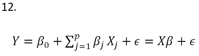
In recent years, several Bayesian linear models have been proposed for genetic studies using the SNP data, including Bayesian sparse linear mixed models, Bayesian spike-and-slab regression models, and Bayesian variable selection models [7]. These models have been used to identify genetic variants associated with complex traits, predict the traits using the SNP data, and identify genetic pathways involved in disease pathogenesis. Note that selecting the best predictors is among the most important aspects of building a linear model. The aim is to find the “best” model based on a subset of predictors, denoted as X1, X2, ..., Xk . The model is written as (Equation 1):
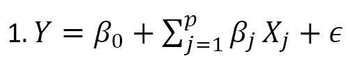
, where p≤k. In genetic studies, selecting the best genetic model (e.g. identification of sensitive and reliable predictors for early detection of cancer cells in clinical trials) is very important [8]. Bayesian model averaging (BMA) addresses this issue by considering a set of candidate models, each of which represents a different hypothesis about the underlying relationship between the response variable and the predictors [9, 10, 11]. Each model assigns a prior probability that reflects the degree of belief in its validity before observing the data. The prior probabilities can be based on prior knowledge or be assigned using the Bayesian model selection technique [12]. The posterior probabilities of the models are used to compute the model-averaged prediction, which is a weighted average of the predictions from each model. This leads to a more robust and reliable prediction, since it considers the uncertainty about the true model [12, 3].
Also, in linear models, the distribution of errors is typically assumed to follow the normal distribution. However, in reality, the assumption of normality may not be appropriate, which is the interest of this study. This article considers the skew-normal and skew-t distributions of errors, and the linear models with these two distributions in the Bayesian framework are introduced. The BMA is used to select the best linear model for the SNP data. In this regard, the numerical studies on real and simulated SNP data are carried out.
Materials and Methods
In this study, the BMA is carried out based on two approaches. The first one is Occam’s window. This method includes averaging over a decreased set of models. The Markov-Chain Monte Carlo model composition (MC3) is the second approach developed by Madigan and York [4]. By this approach, we can estimate the full solution directly for linear regression models. It employs the Markov-Chain Monte Carlo (MCMC) method that generates a process that moves through the model space to approximate the posterior distribution of the variable of interest.
Accounting for model uncertainty using BMA
We know that if a single best model is considered as the true model, inferences based on the model ignore model uncertainty, which can lead to underestimating uncertainty about interested quantities. Leamer [13] proposed a standard Bayesian approach to this issue (Equation 2). Let M={M1, ..., MK} be the set of all models under study that could describe the data, and Δ is the amount of interest, such as a future observation. Given the data D, the posterior distribution of Δ is calculated as:
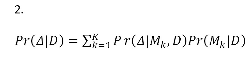
This is a weighted average of the posterior distributions (i.e. BMA). In Equation 2, the posterior probability of the model Mk is obtained as:

Where,

In Equations 3 and 4, Pr(D|Mk) is the marginal likelihood of the model Mk, θk is the parameter of model Mk, Pr(D|θk, Mk) is the prior distribution of θk under the model Mk, Pr(D|θk, Mk) is the likelihood, and Pr(Mk) is the prior probability of the true model Mk. As can be seen, all models are taken in to consideration. Averaging over all the models gives a higher predictive ability than the use of any single model (Mj), since:

In the implementation of BMA, there are two problems: (i) High integrals in Equation 4 make it difficult to compute posterior probabilities; (ii) There are a huge number of models in Equation 2. In the next section, we explain two approaches for solving these problems.
Occam’s window
The first method for accounting for the model uncertainty is Occam’s window [3]. This approach lies in two basic principles:
(i) Discarding the models with fewer predictions: If a model provides less accurate predictions than the best model, it should be neglected and discarded. Therefore, the models that do not belong to the set:

should be removed from Equation 2. In the Equation 6, the C value is determined by the researcher, and maxl Pr(Ml |D) is the model with the highest posterior model probability. Note that the number of models in Occam’s window is augmented as C decreases.
(ii) Occam’s razor application: We remove the models that are supported by the data from their simpler sub-models. In other words, we exclude the models from Equation 2 that belong to the set:

Equation 2 is thus rewritten as:
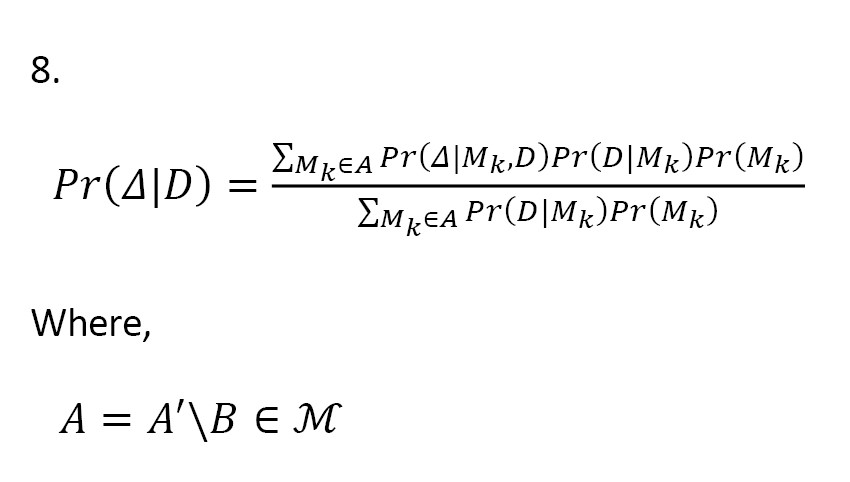
This largely reduces the number of models in Equation 2, and now a search strategy is required to distinguish the models in A.
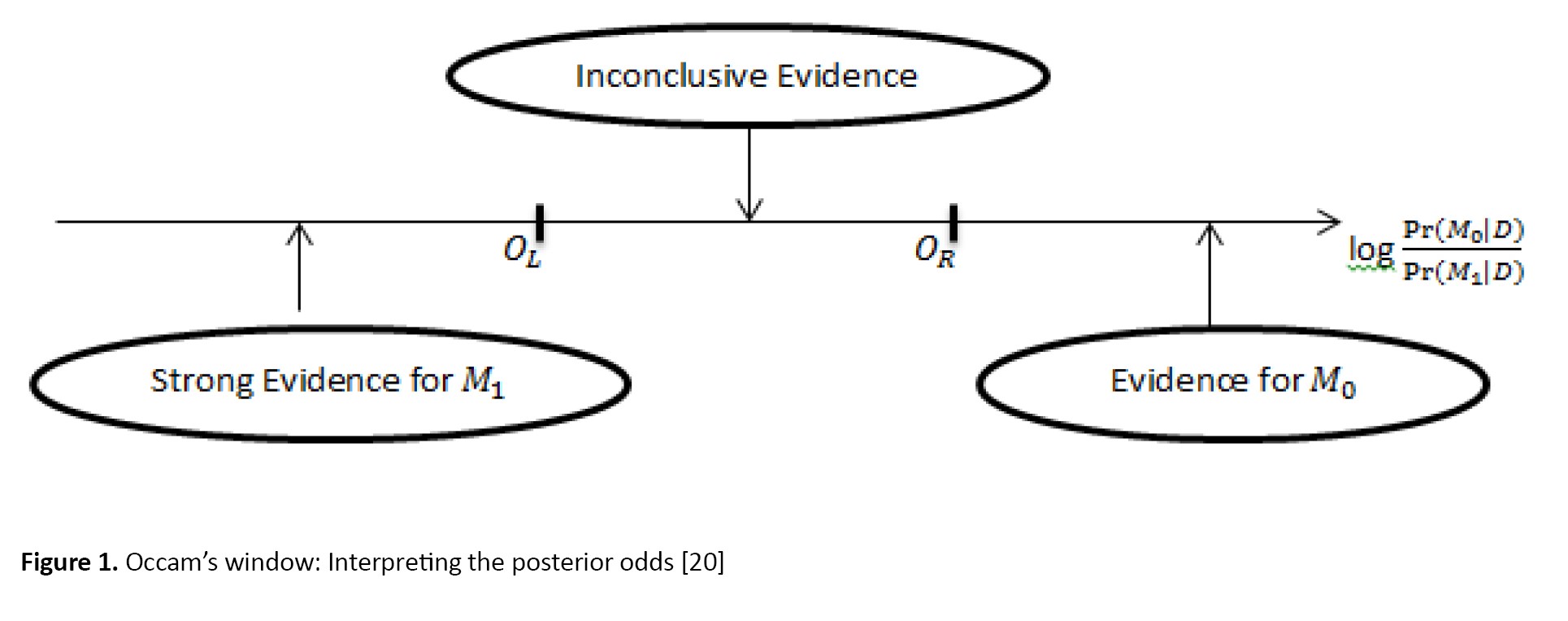
The Occam’s window concerns the interpretation of the ratio of posterior model probabilities (RPM):
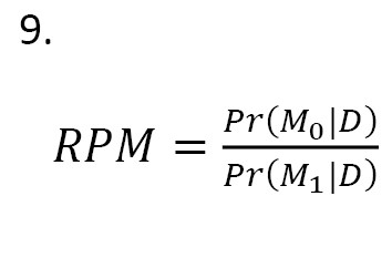
In Equation 9, M0, is a model smaller than the two models and the model M1 is larger. Two models are evaluated based on their PRM. In this regard, we make decisions about the models as:
1. If log(RPM) value is positive (i.e. the given data is an evidence for the smaller model), we reject M1 and consider M0 ;
2. If log(RPM) value is small and negative, we consider both models;
3. If log(RPM) value is large and negative, i.e. smaller than OL=-log(C) where C is defined by the researcher, we reject M0 and consider M1.
The basic concept is shown in Figure 1.
Genetic studies using single nucleotide polymorphisms (SNPs) have been widely used to identify genetic variants associated with complex traits. Bayesian linear models have emerged as a popular tool for analyzing SNP data due to their ability to handle high-dimensional data and their ability to incorporate prior information into the analysis. Bayesian linear models involve finding the relationship between a dependent variable and one or more independent variables, which are also known as predictors or covariates. In genetic studies using the SNP data, the dependent variable is often a complex trait or disease status, and the independent variables are genetic variants, such as SNPs. Bayesian linear models can be used to test the association between the dependent variable and each independent variable when it is controlled by other covariates, such as age, sex, and environmental factors.
Bayesian approach has several advantages over the traditional frequentist approach, including the ability to handle complex models and incorporate prior knowledge or beliefs into the analysis. In genetic studies, the Bayesian approach can be used to utilize prior information on genetic effects or to borrow strength across related traits or populations. One of the key advantages of Bayesian linear models in genetic studies is their ability to account for uncertainty in estimating genetic effects [1-6]. By modeling the uncertainty in the estimates, Bayesian methods can provide more accurate estimates of effect sizes and standard errors, and can also facilitate model selection and hypothesis testing.
In recent years, several Bayesian linear models have been proposed for genetic studies using the SNP data, including Bayesian sparse linear mixed models, Bayesian spike-and-slab regression models, and Bayesian variable selection models [7]. These models have been used to identify genetic variants associated with complex traits, predict the traits using the SNP data, and identify genetic pathways involved in disease pathogenesis. Note that selecting the best predictors is among the most important aspects of building a linear model. The aim is to find the “best” model based on a subset of predictors, denoted as X1, X2, ..., Xk . The model is written as (Equation 1):
, where p≤k. In genetic studies, selecting the best genetic model (e.g. identification of sensitive and reliable predictors for early detection of cancer cells in clinical trials) is very important [8]. Bayesian model averaging (BMA) addresses this issue by considering a set of candidate models, each of which represents a different hypothesis about the underlying relationship between the response variable and the predictors [9, 10, 11]. Each model assigns a prior probability that reflects the degree of belief in its validity before observing the data. The prior probabilities can be based on prior knowledge or be assigned using the Bayesian model selection technique [12]. The posterior probabilities of the models are used to compute the model-averaged prediction, which is a weighted average of the predictions from each model. This leads to a more robust and reliable prediction, since it considers the uncertainty about the true model [12, 3].
Also, in linear models, the distribution of errors is typically assumed to follow the normal distribution. However, in reality, the assumption of normality may not be appropriate, which is the interest of this study. This article considers the skew-normal and skew-t distributions of errors, and the linear models with these two distributions in the Bayesian framework are introduced. The BMA is used to select the best linear model for the SNP data. In this regard, the numerical studies on real and simulated SNP data are carried out.
Materials and Methods
In this study, the BMA is carried out based on two approaches. The first one is Occam’s window. This method includes averaging over a decreased set of models. The Markov-Chain Monte Carlo model composition (MC3) is the second approach developed by Madigan and York [4]. By this approach, we can estimate the full solution directly for linear regression models. It employs the Markov-Chain Monte Carlo (MCMC) method that generates a process that moves through the model space to approximate the posterior distribution of the variable of interest.
Accounting for model uncertainty using BMA
We know that if a single best model is considered as the true model, inferences based on the model ignore model uncertainty, which can lead to underestimating uncertainty about interested quantities. Leamer [13] proposed a standard Bayesian approach to this issue (Equation 2). Let M={M1, ..., MK} be the set of all models under study that could describe the data, and Δ is the amount of interest, such as a future observation. Given the data D, the posterior distribution of Δ is calculated as:
This is a weighted average of the posterior distributions (i.e. BMA). In Equation 2, the posterior probability of the model Mk is obtained as:
Where,
In Equations 3 and 4, Pr(D|Mk) is the marginal likelihood of the model Mk, θk is the parameter of model Mk, Pr(D|θk, Mk) is the prior distribution of θk under the model Mk, Pr(D|θk, Mk) is the likelihood, and Pr(Mk) is the prior probability of the true model Mk. As can be seen, all models are taken in to consideration. Averaging over all the models gives a higher predictive ability than the use of any single model (Mj), since:
In the implementation of BMA, there are two problems: (i) High integrals in Equation 4 make it difficult to compute posterior probabilities; (ii) There are a huge number of models in Equation 2. In the next section, we explain two approaches for solving these problems.
Occam’s window
The first method for accounting for the model uncertainty is Occam’s window [3]. This approach lies in two basic principles:
(i) Discarding the models with fewer predictions: If a model provides less accurate predictions than the best model, it should be neglected and discarded. Therefore, the models that do not belong to the set:
should be removed from Equation 2. In the Equation 6, the C value is determined by the researcher, and maxl Pr(Ml |D) is the model with the highest posterior model probability. Note that the number of models in Occam’s window is augmented as C decreases.
(ii) Occam’s razor application: We remove the models that are supported by the data from their simpler sub-models. In other words, we exclude the models from Equation 2 that belong to the set:
Equation 2 is thus rewritten as:
This largely reduces the number of models in Equation 2, and now a search strategy is required to distinguish the models in A.
The Occam’s window concerns the interpretation of the ratio of posterior model probabilities (RPM):
In Equation 9, M0, is a model smaller than the two models and the model M1 is larger. Two models are evaluated based on their PRM. In this regard, we make decisions about the models as:
1. If log(RPM) value is positive (i.e. the given data is an evidence for the smaller model), we reject M1 and consider M0 ;
2. If log(RPM) value is small and negative, we consider both models;
3. If log(RPM) value is large and negative, i.e. smaller than OL=-log(C) where C is defined by the researcher, we reject M0 and consider M1.
The basic concept is shown in Figure 1.
Madigan and Raftery [3] gave a detailed description of Occam’s window algorithm and showed how averaging over the selected models gives better predictive performance than any single model in each of the considered cases.
Markov-Chain Monte Carlo model composition
In the MC3 method, the MCMC approach is used to approximate Equation 2 [14]. A modified version of the MC3 method adopted from Madigan and York [4] is used in this study, which generates a stochastic process that moves through model space. A Markov chain M(t), t=1, 2,... with state space M and equilibrium distribution Pr(Mi|D) can be constructed. If this Markov chain is simulated for t=1, . . . , N, under certain regularity conditions, for any function f(Mi) defined on M, the average:
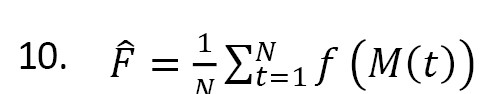
is an estimate of E(f(M)) as N→∞ [12]. To compute Equation 2 by this approach, set f(M)=Pr(Δ|M,D). To construct the Markov chain, for each M ϵ M, a neighborhood nbd(M) is defined that includes the model M itself and the set of models with one edge more or fewer than M. Its transition matrix q is defined by setting q(M→M' )=0 for all M' ϵ nbd(M) and q(M→M')≠0, constant for all M'ϵnbd(M). If the chain is in state M, we access to state M' by considering q(M→M'). It is accepted with probability: ; otherwise, we do not move from state M [4].
Bayesian framework
In this section, two linear models are presented whose errors follow some skew distributions. The first model is concerned with skew-normal error distribution and the second model considers the skew-t distribution.
Errors with skew-normal distribution
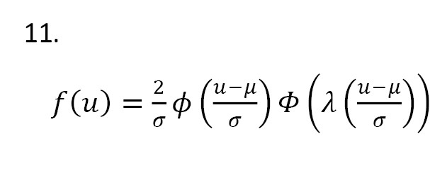
Let U has a skew-normal distribution with the shape parameter λ ϵ R, mean μ ϵ R, and standard deviation σ ϵ R+, denoted by SN(μ,σ,λ). The probability density function (PDF) of U is defined as Equation 11:
Azzalini and Capitanio [15] proposed a simple linear regression model where the error terms are independent and identically distributed from SN(0,1,λ). Consider the model (Equation 12):
where X is a n×(p+1) matrix that contains the observation of predictors, and ϵ=(ϵ1,...,ϵn)' and Y=(Y1,...,Yn)' are n×1 vectors of errors and dependent variable observation, respectively. Also, β is a (p+1)1 vector of coefficients. Let ϵi ~ SN(0,1,λ) and independent for i=1,..,n. The likelihood function for Equation 12 is written as Equation 13:
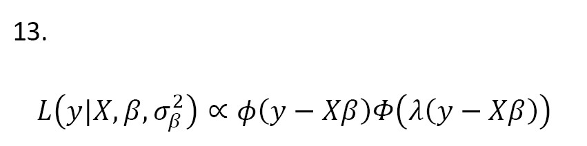
where ϕ(.) and ϕ(.) are the PDF and cumulative density function (CDF) of the standard normal distribution, respectively. Assume
[16]. Then, the joint prior distribution is:
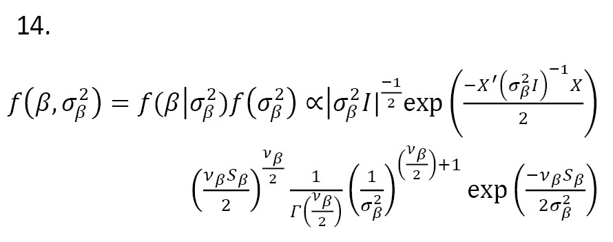
If the errors have a skew-normal distribution
ϵ ~ SN(μ,σ,λ), the posterior distribution is obtained as:

The posterior distribution leads to estimate the model parameters.
Errors with skew-t distribution
Let U ~ SN(0,1,λ) and , U and Z are independent. Then, the random variable X= has the skew-t distribution with shape parameter λ ϵ R and degrees of freedom r>0. The PDF of X is obtained as :

where t(;) and T(;) are the PDF and CDF of the t distribution, respectively [17, 18]. Now, suppose Equation 16 with errors from the skew-t distribution, i.e. ϵ ~ STrϵ (λ), where rϵ represents the degree of freedom . The likelihood function for Equation 16 is written as (Equation 17):

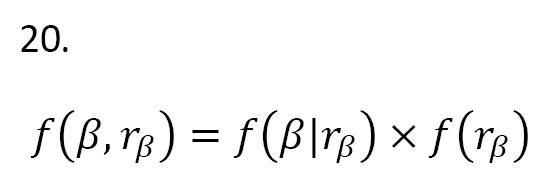
Let β have the p-variate t distribution with degrees of freedom rβ, mean vector μβ, and correlation matrix R, denoted by MVTrβ (μβ,R). Its PDF is obtained as:

Here, assume that rβ has a truncated t distribution with degrees of freedom r :

where I(.) is an indicator function, α0=T(b;r)-T(a;r) is a normalizing constant with -∞[19]. Then, the joint prior distribution is defined:
In the Equation 21, μ and are set 0 and respectively. Therefore, the posterior distribution P(β,rβ |Data) is given as:

The above formula provides more information about parameters and their estimates.
Numerical study
In this study, we evaluated the performance of the BMA method for linear models with skew-normal and skew-t errors. This evaluation was carried out on both simulated and real data. To select the best model, Occam’s window and MC3 method were used. The computations were carried out in R software, version 4.4.0.
Results
Numerical study on simulated data
At first, to assess the performance of the BMA method, we simulated data from linear models with skew-normal and skew-t distributed errors.
Case 1. We assess the effect of model averaging on prediction performance under a little model uncertainty. We simulated 6 predictors for 100 observations from the standard normal distribution. We obtained the response values using the following model (Equation 22):

where ϵ ~ SN100 (0, 1, 2.8). Based on Occam’s window and MC3 method, we tried to find the best model. The models the highest posterior probability are presented in Tables 1 and 2.


For each model, the included independent variables are specified. The posterior probability corresponds to the validity of each model when errors have skew-normal distribution. Based on Occam’s window, the best model was X6 (Table 1), while based on the MC3 method the models X4 and X5 were yielded as the best model (Table 2). Therefore, the MC3 method gives the true model (Equation 22). The models X4 and X5 proposed by the MC3 method had a probability value of 1, indicating the importance of these variables.
Case 2. We simulated 6 predictors for observations from a standard normal distribution. The response values are obtained from the following model (Equation 23):
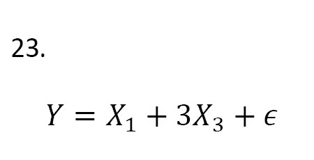
where ϵ ~ ST100 (0,1,0,2). The results are shown in Tables 3 and 4.
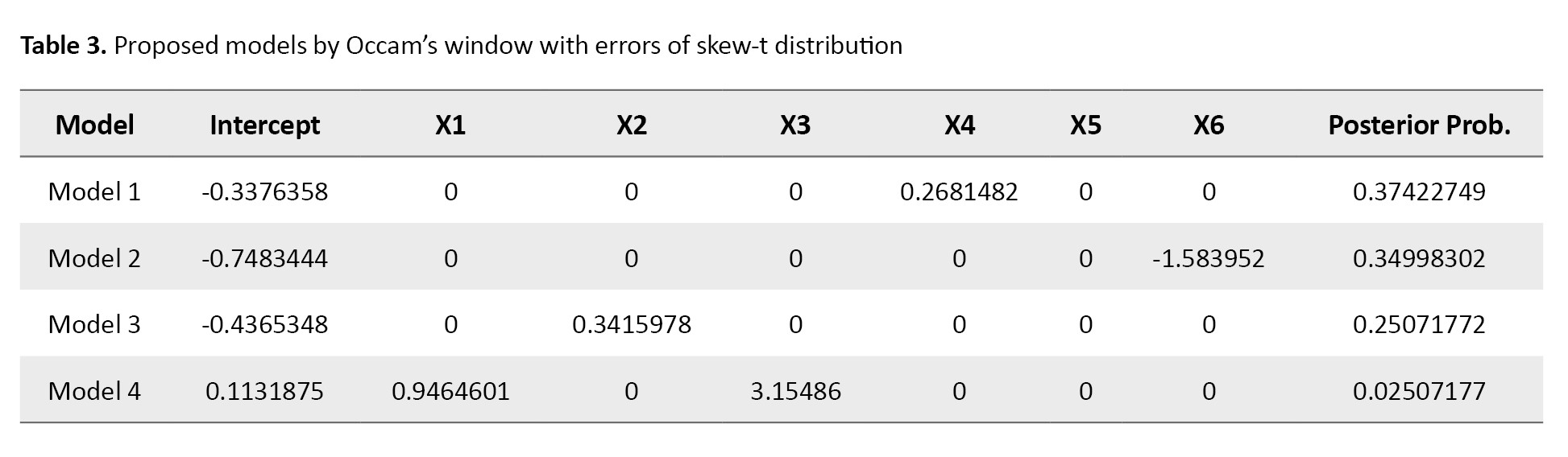
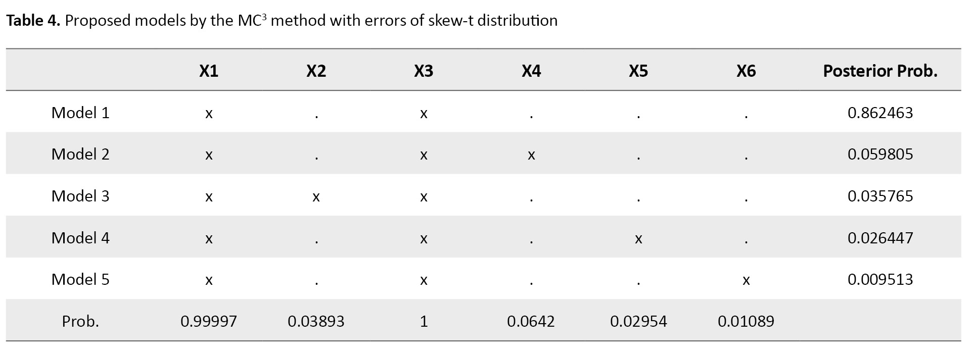
As can be seen, based on Occam’s window, the best model was according to its posterior probability value (Table 3), which is different from the true model (Equation 23). The MC3 method showed that the models X1 and X3 had the highest probability value (Table 4). Therefore, the MC3 method proposes the true model and outperforms Occam’s window. Overall, we can conclude that the MC3 method works better than Occam’s window and gives a high posterior probability to the best model.
Numerical study on real data
Rice SNP-Seek Database was used to obtain real data. The data consists of information from 152 SNPs with 6 phenotypes. It is interesting to study the relationship between SNP (stock ID) and phenotypes CUST REPRO (culm strength at reproductive - cultivated), FLA EREPRO (flag leaf (attitude of the blade) - early observation), FLA REPRO (flag leaf angle at reproductive - cultivated), INCO REV REPRO (internode color at reproductive - cultivated), LA (leaf angle - cultivated), LPCO REV POST (Lemma and palea color at post-harvest).
Assuming that the errors had a skew-normal and skew-t distribution, the BMA method was employed to select the best model for the two cases mentioned in the previous section. The results related to the skew-normal distribution are presented in Tables 5 and 6.


Tables 7 and 8 show the results related to the skew-t distribution.
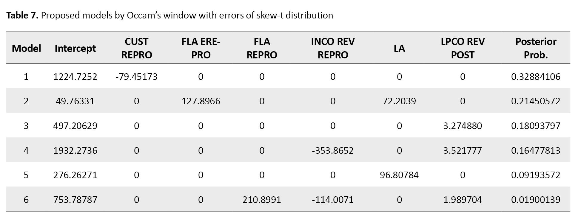

Occam’s window method selected CUST REPRO variable in the best model under skew-normal and skew-t distributions (Tables 5 and 7). While the MC3 method showed that the best model contained FLA EREPRO and LA data when the errors had either skew-normal or skew-t distribution (Tables 6 and 8). Based on the posterior probability value, it is more plausible that the model proposed by the MC3 method was the true model. Figure 2 shows the best selected models by Occam’s window for errors with skew-normal and skew-t distributions.
Markov-Chain Monte Carlo model composition
In the MC3 method, the MCMC approach is used to approximate Equation 2 [14]. A modified version of the MC3 method adopted from Madigan and York [4] is used in this study, which generates a stochastic process that moves through model space. A Markov chain M(t), t=1, 2,... with state space M and equilibrium distribution Pr(Mi|D) can be constructed. If this Markov chain is simulated for t=1, . . . , N, under certain regularity conditions, for any function f(Mi) defined on M, the average:
is an estimate of E(f(M)) as N→∞ [12]. To compute Equation 2 by this approach, set f(M)=Pr(Δ|M,D). To construct the Markov chain, for each M ϵ M, a neighborhood nbd(M) is defined that includes the model M itself and the set of models with one edge more or fewer than M. Its transition matrix q is defined by setting q(M→M' )=0 for all M' ϵ nbd(M) and q(M→M')≠0, constant for all M'ϵnbd(M). If the chain is in state M, we access to state M' by considering q(M→M'). It is accepted with probability: ; otherwise, we do not move from state M [4].
Bayesian framework
In this section, two linear models are presented whose errors follow some skew distributions. The first model is concerned with skew-normal error distribution and the second model considers the skew-t distribution.
Errors with skew-normal distribution
Let U has a skew-normal distribution with the shape parameter λ ϵ R, mean μ ϵ R, and standard deviation σ ϵ R+, denoted by SN(μ,σ,λ). The probability density function (PDF) of U is defined as Equation 11:
Azzalini and Capitanio [15] proposed a simple linear regression model where the error terms are independent and identically distributed from SN(0,1,λ). Consider the model (Equation 12):
where X is a n×(p+1) matrix that contains the observation of predictors, and ϵ=(ϵ1,...,ϵn)' and Y=(Y1,...,Yn)' are n×1 vectors of errors and dependent variable observation, respectively. Also, β is a (p+1)1 vector of coefficients. Let ϵi ~ SN(0,1,λ) and independent for i=1,..,n. The likelihood function for Equation 12 is written as Equation 13:
where ϕ(.) and ϕ(.) are the PDF and cumulative density function (CDF) of the standard normal distribution, respectively. Assume
[16]. Then, the joint prior distribution is:
If the errors have a skew-normal distribution
ϵ ~ SN(μ,σ,λ), the posterior distribution is obtained as:
The posterior distribution leads to estimate the model parameters.
Errors with skew-t distribution
Let U ~ SN(0,1,λ) and , U and Z are independent. Then, the random variable X= has the skew-t distribution with shape parameter λ ϵ R and degrees of freedom r>0. The PDF of X is obtained as :
where t(;) and T(;) are the PDF and CDF of the t distribution, respectively [17, 18]. Now, suppose Equation 16 with errors from the skew-t distribution, i.e. ϵ ~ STrϵ (λ), where rϵ represents the degree of freedom . The likelihood function for Equation 16 is written as (Equation 17):
Let β have the p-variate t distribution with degrees of freedom rβ, mean vector μβ, and correlation matrix R, denoted by MVTrβ (μβ,R). Its PDF is obtained as:
Here, assume that rβ has a truncated t distribution with degrees of freedom r :
where I(.) is an indicator function, α0=T(b;r)-T(a;r) is a normalizing constant with -∞[
In the Equation 21, μ and are set 0 and respectively. Therefore, the posterior distribution P(β,rβ |Data) is given as:
The above formula provides more information about parameters and their estimates.
Numerical study
In this study, we evaluated the performance of the BMA method for linear models with skew-normal and skew-t errors. This evaluation was carried out on both simulated and real data. To select the best model, Occam’s window and MC3 method were used. The computations were carried out in R software, version 4.4.0.
Results
Numerical study on simulated data
At first, to assess the performance of the BMA method, we simulated data from linear models with skew-normal and skew-t distributed errors.
Case 1. We assess the effect of model averaging on prediction performance under a little model uncertainty. We simulated 6 predictors for 100 observations from the standard normal distribution. We obtained the response values using the following model (Equation 22):
where ϵ ~ SN100 (0, 1, 2.8). Based on Occam’s window and MC3 method, we tried to find the best model. The models the highest posterior probability are presented in Tables 1 and 2.
For each model, the included independent variables are specified. The posterior probability corresponds to the validity of each model when errors have skew-normal distribution. Based on Occam’s window, the best model was X6 (Table 1), while based on the MC3 method the models X4 and X5 were yielded as the best model (Table 2). Therefore, the MC3 method gives the true model (Equation 22). The models X4 and X5 proposed by the MC3 method had a probability value of 1, indicating the importance of these variables.
Case 2. We simulated 6 predictors for observations from a standard normal distribution. The response values are obtained from the following model (Equation 23):
where ϵ ~ ST100 (0,1,0,2). The results are shown in Tables 3 and 4.
As can be seen, based on Occam’s window, the best model was according to its posterior probability value (Table 3), which is different from the true model (Equation 23). The MC3 method showed that the models X1 and X3 had the highest probability value (Table 4). Therefore, the MC3 method proposes the true model and outperforms Occam’s window. Overall, we can conclude that the MC3 method works better than Occam’s window and gives a high posterior probability to the best model.
Numerical study on real data
Rice SNP-Seek Database was used to obtain real data. The data consists of information from 152 SNPs with 6 phenotypes. It is interesting to study the relationship between SNP (stock ID) and phenotypes CUST REPRO (culm strength at reproductive - cultivated), FLA EREPRO (flag leaf (attitude of the blade) - early observation), FLA REPRO (flag leaf angle at reproductive - cultivated), INCO REV REPRO (internode color at reproductive - cultivated), LA (leaf angle - cultivated), LPCO REV POST (Lemma and palea color at post-harvest).
Assuming that the errors had a skew-normal and skew-t distribution, the BMA method was employed to select the best model for the two cases mentioned in the previous section. The results related to the skew-normal distribution are presented in Tables 5 and 6.
Tables 7 and 8 show the results related to the skew-t distribution.
Occam’s window method selected CUST REPRO variable in the best model under skew-normal and skew-t distributions (Tables 5 and 7). While the MC3 method showed that the best model contained FLA EREPRO and LA data when the errors had either skew-normal or skew-t distribution (Tables 6 and 8). Based on the posterior probability value, it is more plausible that the model proposed by the MC3 method was the true model. Figure 2 shows the best selected models by Occam’s window for errors with skew-normal and skew-t distributions.
Discussion
In the context of Bayesian inference, selecting the best model is a critical challenge, particularly in situations with a multitude of potential predictors. The BMA method is a powerful approach to address this issue by effectively managing the uncertainties about the model and its parameters. This becomes more pivotal when one considers the vast number of possible linear models with countless predictors. The literature, including the work of Raftery et al., has shown the use of BMA in standard linear regression contexts, particularly when errors have normal distribution [20]. However, in many real-world scenarios, the errors may not have normal distribution, as many datasets exhibit skewness in the distribution of their errors. The adaptability of the BMA method to such complex scenarios is noteworthy, especially when it comes to identifying the most appropriate subset of predictors under these non-normal distributions, such as skew-normal and skew-t distributions. By employing the BMA method alongside techniques such as Occam’s Window and MC3, researchers are able to navigate the vast space of models and quantify and manage their uncertainties effectively. Occam’s window provides a streamlined approach to model selection by considering the simplicity principle, and MC3 allows for the extensive exploration of the model space, albeit with greater computational demands. Each method contributes distinctly to the model selection process, enabling researchers to weigh the trade-offs between computational efficiency and model accuracy. The integration of BMA with these techniques underscores the importance of identifying a single best model and recognizing the importance of multiple competing models within the context of uncertainty. This perspective is essential in biological and ecological studies where underlying processes may be inherently complex and multifactorial. Overall, the use of BMA along with strategies that address the nuances of error distributions equips researchers with robust tools to draw more accurate inferences and predictions from their models, thereby enhancing the reliability of their biological insights. As the field continues to evolve, embracing such advanced methodologies will be vital for addressing the intricate challenges presented by biological data.
Conclusion
Based on the analysis of genetic data from 3000 rice varieties, this study highlights the effectiveness and applicability of two model selection methods (Occam’s Window and MC3) in understanding the relationship between genotype and phenotype. Although both methods are suitable for inference and prediction in biostatistical contexts, the MC3 method is more capable to identify the true model with greater accuracy, particularly when dealing with skew distributions. Although Occam’s Window completes its computations more rapidly, it tends to rank lower in model accuracy compared to MC3.This suggests that researchers in the field of biology and genetics should consider using the MC3 method for complex genetic modeling, despite its longer computation time, since it provides more reliable insights into the underlying genetic factors influencing phenotypic variation in rice varieties. The findings emphasize the importance of employing robust modeling approaches in biological research to enhance our understanding of genetic diversity and its implications for crop improvement.
Ethical Considerations
Compliance with ethical guidelines
There were no ethical considerations to be considered in this research.
Funding
This research did not receive any grant from funding agencies in the public, commercial, or non-profit sectors.
Authors contributions
All authors equally contribute to preparing all parts of the research.
Conflict of interest
The authors declared no conflict of interest.
References
- Draper D. Assessment and propagation of model uncertainty (with discussion). Journal of the Royal Statistical Society: Series B (Methodological). 1995; 57(1):45-97. [DOI: 10.1111/j.2517-6161.1995.tb02015.x]
- Jacobovic R. On the relation between the true and sample correlations under bayesian modelling of gene expression datasets. Statistical Applications in Genetics and Molecular Biology. 2018; 17(4). [DOI:10.1515/sagmb-2017-0068] [PMID]
- Madigan D, Raftery AE. Model selection and accounting for model uncertainty in graphical models using occam's window. American Statistical Association. 1994; 89 (428):1535-46. [DOI: 10.1080/01621459.1994.10476894]
- Madigan D, York J. Bayesian graphical models for discrete data. International Statistical Review. 1995; 63(2): 15-32. [DOI:10.2307/1403615]
- Raftery AE. Bayesian model selection in social research. Sociological Methodology. 1995; 25:111-63. [Link]
- Stephens M, Balding DJ. Bayesian statistical methods for genetic association studies. . Nature Reviews Genetics. 2009; 10(10):681-90. [DOI: 10.1038/nrg2615]
- Koch B, Vock DM, Wolfson J, Vock LB. Variable selection and estimation in causal inference using Bayesian spike and slab priors. Statistical Methods in Medical Research. 2020;29(9):2445-2469. [DOI:10.1177/0962280219898497]
- Hocking RR. A biometrics invited paper. The analysis and selection of variables in linear regression. Biometrics. 1976: 32(1):1-49. [DOI:10.2307/2529336]
- George EI, McCulloch RE. Variable selection via gibbs sampling. American Statistical Association. 1993; 88(423):881-890. [DOI: 10.1080/01621459.1993.10476353]
- Kass RE, Raftery AE. Bayes factors. Journal of the American Statistical Association. 1995; 90(430):773-95. [DOI:10.2307/2291091]
- Miller AJ. Selection of subsets of regression variables (with discussion). Journal of the Royal Statistical Society. Series A (General). 1984; 147(3):389-425. [DOI:10.2307/2981576]
- Hoeting JA, Madigan D, Raftery AE, Volinsky Ch. Bayesian model averaging: A Tutorial. Statistical Science. 1999; 14(4):382-417.
- Leamer EE. Specification searches. New York: Wiley; 1978. [Link]
- Smith A, Roberts G. Bayesian computation via gibbs sampler and related markov chain monte carlo methods. Royal Statistical Society, Ser. B. 1993; 55(1):3-23. [DOI:10.1111/j.2517-6161.1993.tb01466.x]
- Azzalini A, Capitanio A. The skew-normal and related families, 1999. [DOI: 10.1017/CBO9781139248891]
- Sorensen D, Gianola D. Likelihood, Bayesian, and MCMC methods in quantitative genetics. New York: Springer; 2002. [DOI:10.1007/b98952]
- Azzalini A, Capitanio A. Distributions generated by perturbation of symmetry with emphasis on a multivariate skew t-distribution. Journal of the Royal Statistical Society Series B: Statistical Methodology. 2003; 65(2):367-89. [DOI:10.1111/1467-9868.00391]
- Azzalini A, Capitanio A. The skew-normal and related families. Cambridge: Cambridge University Press; 2013. [DOI:10.1017/CBO9781139248891]
- Ho HJ, . Lin TI, Chen HY, Wang WL. Some results on the truncated multivariate t distribution. Journal of Statistical Planning and Inference. 2012; 142(1):25-40. [DOI:10.1016/j.jspi.2011.06.006]
- Raftery AE, Madigan D, Hoeting JA. Bayesian model averaging for linear regression models. Journal of the American Statistical Association. 2014; 92(437):179-91. [DOI:10.1080/01621459.1997.10473615]
Type of Study: Original Article |
Subject:
Biostatistics
Send email to the article author
| Rights and permissions | |
 |
This work is licensed under a Creative Commons Attribution-NonCommercial 4.0 International License. |

This is an open access article distributed under the terms of the Creative Commons Attribution License (CC-By-NC), which permits use, distribution, and reproduction in any medium, provided the original work is properly cited and is not used for commercial purposes.
Contact Information
